Data Science Methodology Class 12 Notes – The CBSE has updated the syllabus for St. XII (Code 843). The NCERT notes are made based on the updated CBSE textbook. All the important information is taken from the Artificial Intelligence Class XII Textbook Based on the CBSE Board Pattern.
Data Science Methodology Class 12 Notes
Data science methodology
A data science methodology is a structured approach to solving problems. A methodology gives the data scientist a framework for designing an AI project. The framework will help the team to decide on the methods, processes, and strategies that will be employed to obtain the correct output required from the AI project.
Definition: Data Science Methodology is a process with a prescribed sequence of iterative steps that data scientists follow to approach a problem and find a solution.
Data Science Methodology which was introduced by John Rollins, a Data Scientist at IBM Analytics. It consists of 10 steps. The technique is broken down into five modules, each of which covers two stages and explains why each is necessary.
- From Problem to Approach
- From Requirements to Collection
- From Understanding to Preparation
- From Modelling to Evaluation
- From Deployment to Feedback
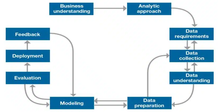
1. Business understanding
In the first stage, we have to understand the problem and try to comprehend what is exactly required in the business. This is also known as problem scoping and defining. The term can use the 5W1H Problem Canvas to deeply understand the issue. This stage also involves using the Design Thinking Framework.
To solve a problem, it’s crucial to understand the customer’s needs. This can be achieved by asking relevant questions and engaging in discussions with all stakeholders.
2. Analytic Approach
In this stage, the data scientist identifies and collects the questions or clarification from the stakeholders which is required for analysis. In this stage data scientist involves asking more questions to stakeholders so that the AI project team can decide on the correct approach to solve the problem.
To solve a particular problem, there are four main types of data analytics.
- Descriptive Analytics
- Diagnostic Analytics
- Predictive Analytics
- Prescriptive Analytics
Descriptive Analytics: Descriptive analytics summarizes the past data to identify trends and patterns. Descriptive analysitics use tools like graphs, charts and statistical measures like mean, median, mode to understand the data. For example: To calculate the average marks of students in an exam or analyzing sales data from the previous year.
Diagnostic Analystics: Diagnostic analytics understand the reason behind why some things have happened. Diagnostic analytics analyze past data using techniques like root cause analysis, hypothesis testing, correlation analysis, etc. For example, if the sales of a company dropped, diagnostic analysis will help to find the cause for it by analyzing questions like “Is it due to poor customer service?” or “low product quality?”
Predictive Analytics: This analytics uses the past data to make predictions about future events or trends, using techniques like regression, classification, clustering, etc. The main purpose is to foresee future outcomes and make informed decisions. For example, a company can use predictive analytics to forecast its sales, demand, inventory, customer purchase patterns, etc., based on previous sales data.
Prescriptive Analytics: Prescriptive analytics is a data-driven approach in machine learning and statistical algorithms to recommend actions that can improve business outcomes. The techniques used in prescriptive analytics are optimization, simulation, decision analysis, etc. For example, to design the right strategy to increase the sales during festival season by analyzing past data and thus optimize pricing, marketing, production, etc.
We can summarize each of these analytics as given in Table
| Descriptive Analytics | Diagnostic Analytics | Predictive Analytics | Prescriptive Analytics | |
|---|---|---|---|---|
| Focus | Questions on summarizing historical data | Questions on understanding why certain events occurred | Questions on predicting future outcomes based on historical data patterns | Questions on determining the best course of action |
| Purpose | Identify patterns, trends, and anomalies in past data | Uncover root causes and factors contributing to specific outcomes | Forecast future events or behaviors | Recommend specific actions or interventions based on predictive insights. May indirectly influence classification through recommendations |
3. Data requirements
In data requirements, the 5W1H questioning method is used to identify the data requirements and also wants to find the purpose of data. Data requirements understand the steps involved in the processes that create, read, update, or delete data and determine the correct use of data.
Determining the specific information needed for our analysis or project includes:
- Identifying the types of data required, such as numbers, words, or images.
- Considering the structure in which the data should be organized, whether it is in a table, text file, or database.
- Identifying the sources from which we can collect the data, and
- Any necessary cleaning or organization steps required before beginning the analysis.
4. Data collection
Data collection is a process where the data is collected from different sources; it is a fundamental step in data science. Data requirements are decision-makers deciding whether the data collected from different sources requires more or less data. There are mainly two sources of data collection:
- Primary data source: Primary data is raw and unprocessed data that is collected from the original source, like direct observation, experimentation, surveys, interviews, or other methods.
- Secondary data source: Secondary data is ready-to-use data. Secondary data sources refer to the data that is already stored in different areas, like web scraping, databases, social media data, satellite data, etc.
5. Data Understanding
Data understanding is a process where we want to understand if the collected data can solve the problem or not. We also want to check the relevance of the data and want to identify that the data can address the specific problem or question that is going to be evaluated.
6. Data preparation
This stage covers all the activities to build the set of data that will be used in the modelling step. Data is transformed into a state where it is easier to work with. Data preparation includes
- Cleaning of data (dealing with invalid or missing values, removal of duplicate values and assigning a suitable format)
- Combine data from multiple sources (archives, tables and platforms)
- Transform data into meaningful input variables
7. AI modelling
AI modeling is a method of creating algorithms or models that can learn and make intelligent decisions without human intervention. The modeling stage uses the initial version of the dataset prepared and focuses on developing models according to the analytical approach previously defined. Data modeling focuses on developing models that are either descriptive or predictive.
Descriptive Modeling: It is a concept in data science and statistics that focuses on summarizing and understanding the characteristics of a dataset without making predictions or decisions. This includes summarizing the main characteristics, patterns, and trends that are present in the data.
Common Descriptive Techniques:
Summary Statistics: This includes measures like:
- Mean (average), Median, Mode
- Standard deviation, Variance
- Range (difference between the highest and lowest values)
- Percentiles (e.g., quartiles)
Visualizations: Graphs and charts to represent the data, such as:
- Bar charts
- Histograms
- Pie charts
- Box plots
- Scatter plots
Predictive modeling: It involves using data and statistical algorithms to identify patterns and trends in order to predict future outcomes or values. It relies on historical data and uses it to create a model that can predict future behavior or trends or forecast what might happen next. It involves techniques like regression, classification, and time-series forecasting, and can be applied in a variety of fields, from predicting exam scores to forecasting weather or stock prices.
8. Evaluation
Evaluation in an AI project cycle is the process of assessing how well a model performs after training. It involves using test data to measure metrics like accuracy, precision, recall, or F1 score. This helps determine if the model is reliable and effective before deploying it in real-world situations.
Model evaluation can have two main phases.
First phase – Diagnostic measures
It is used to ensure the model is working as intended. If the model is a predictive model, a decision tree can be used to evaluate the output of the model, check whether it is aligned to the initial design or requires any adjustments.
Second phase – Statistical significance test
This type of evaluation can be applied to the model to verify that it accurately processes and interprets the data. This is designed to avoid unnecessary second guessing when the answer is revealed.
9. Deployment
Deployment refers to the stage where the trained AI model is made available to the users in real-world applications. Once the model is evaluated and the data scientist is confident it will work, it is deployed and put to the ultimate test.
10. Feedback
The last stage in the data science methodology is feedback. Feedback from the users will help to refine the model and assess it for performance and impact. Feedback from users can be received in many ways.

Model Validation
Model validation is a process that evaluates the performance and reliability of a model. Model Validation offers a systematic approach to measure its accuracy and reliability, providing insights into how well it generalizes to new, unseen data. The benefits of Model Validation include
- Enhancing the model quality.
- Reduced risk of errors
- Prevents the model from overfitting and underfitting.
Model Validation Techniques
The commonly used Validation techniques are Train-test split, K-Fold Cross Validation, Leave One out Cross Validation, Time Series Cross Validation etc. Let’s discuss the Train test split and K-Fold Cross Validation.
Train Test Split
The train-test split is a technique for evaluating the performance of a machine learning algorithm. It can be used for classification or regression problems and can be used for any supervised learning algorithm.
The procedure involves taking a dataset and dividing it into two subsets, The first subset is used to train the model and is referred to as the training dataset. The second subset is used to test the model.
- Train Dataset: Used to fit the machine learning model.
- Test Dataset: Used to evaluate the fit machine learning model.
How to Configure the Train-Test Split
The parameter is used for the size of the train and test datasets, normally represented as percentages. For example, if 67% of data is allocated for training, then 33% is reserved for testing. The training and testing split depends on the project goal.
Common split percentages include:
● Train: 80%, Test: 20%
● Train: 70%, Test: 30%
● Train: 67%, Test: 33%
K-Fold Cross Validation
K-Fold cross-validation is a technique that splits a dataset into subsets, or folds, to evaluate the model’s performance. For example, suppose you have 100 data points you want to evaluate using K-Fold cross-validation.
- Step 1: Divide the 100 data points into 5 equal parts (folds), each containing 20 data points.
- Step 2: Use the 1st fold as the test set and the remaining 4 folds as the training set.
- Step 3: Use the 2nd fold as the test set, and the remaining 4 will be the training set.
- Step 4: Continue the above steps until each fold has been used as the test set once.
Use the performance metric like accuracy and F1 score to find the final average of these metrics to get the overall model performance.
Difference between Train-Test Split and Cross Validation
| Train-Test Split | Cross Validation |
|---|---|
| Normally applied on large datasets | Normally applied on small datasets |
| Divides the data into training data set and testing dataset. | Divides a dataset into subsets (folds), trains the model on some folds, and evaluates its performance on the remaining data. |
| Clear demarcation on training data and testing data. | Every data point at some stage could be in either testing or training data set. |
MODEL PERFORMANCE – EVALUATION METRICS
Evaluation metrics are used to check the performance and effectiveness of the machine learning model. Evaluation metrics help to compare different models to identify the best-performing one for a specific task. The evaluation matrix is categorized into classification problems and regression problems.
- Classification Problems: The target variable is divided into distinct classes. Metrics include accuracy, precision, recall, F1-score, and AUC-ROC.
- Regression Problems: The target variable is continuous. Metrics include mean squared error (MSE), mean absolute error (MAE), and R-squared.
Evaluation Metrics for Classification
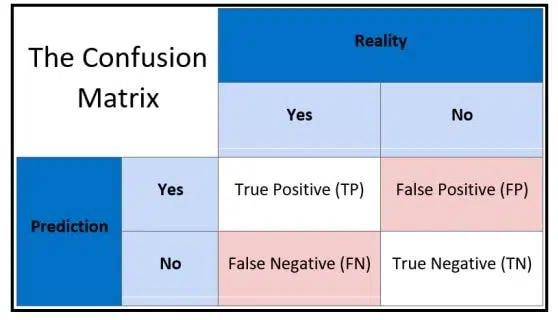
Confusion Matrix
A Confusion Matrix is used to evaluate the performance of a classification model. It summarizes the predictions against the actual outcomes. It creates an N X N matrix, where N is the number of classes or categories that are to be predicted. Suppose there is a problem, which is a binary classification, then N=2 (Yes/No). It will create a 2×2 matrix.
- True Positives: It is the case where the model predicted Yes and the real output was also yes.
- True Negatives: It is the case where the model predicted No and the real output was also No.
- False Positives: It is the case where the model predicted Yes but it was actually No.
- False Negatives: It is the case where the model predicted No but it was actually Yes.
Precision and Recall
Precision measures “What proportion of predicted Positives is truly Positive?”
Precision = (TP)/(TP+FP).
Precision should be as high as possible.
Recall measures “What proportion of actual Positives is correctly classified?”
Recall = (TP)/(TP+FN)
F1-score
A good F1 score means that you have low false positives and low false negatives, so you’re
correctly identifying real threats, and you are not disturbed by false alarms. An F1 score is
considered perfect when it is 1, while the model is a total failure when it is 0.
F1 = 2* (precision * recall)/(precision + recall)
Accuracy
Accuracy = Number of correct predictions / Total number of predictions
Accuracy = (TP+TN)/(TP+FP+FN+TN)
Evaluation Metrics for Regression
MAE (Mean Absolute Error)
Mean Absolute Error is a sum of the absolute differences between predictions and actual values. A value of 0 indicates no error or perfect predictions
MSE (Mean Square Error)
Mean Square Error (MSE) is the most commonly used metric to evaluate the performance of a regression model. MSE is the mean(average) of squared distances between our target variable and predicted values.

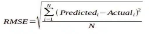
RMSE (Root Mean Square Error)
Root Mean Square Error (RMSE) is the standard deviation of the residuals (prediction errors). RMSE is often preferred over MSE because it is easier to interpret since it is in the same units as the target variable.
Disclaimer: We have taken an effort to provide you with the accurate handout of “Data Science Methodology Class 12 Notes“. If you feel that there is any error or mistake, please contact me at anuraganand2017@gmail.com. The above CBSE study material present on our websites is for education purpose, not our copyrights. All the above content and Screenshot are taken from Artificial Intelligence Class 12 CBSE Textbook, Sample Paper, Old Sample Paper, Board Paper and Support Material which is present in CBSEACADEMIC website, This Textbook and Support Material are legally copyright by Central Board of Secondary Education. We are only providing a medium and helping the students to improve the performances in the examination.
Images and content shown above are the property of individual organizations and are used here for reference purposes only.
For more information, refer to the official CBSE textbooks available at cbseacademic.nic.in