Basic ICT Skills Class 12 Notes

Teachers and Examiners (CBSESkillEduction) collaborated to create the Basic ICT Skills Class 12 Notes. All the important Information are taken from the NCERT Textbook Employability Skills as per the board pattern.

Contents show

basic ict skills class 12 MM2 — Image Source – CBSE | Image by – cbseacademic.nic.in

Performing Tabulation Using Spreadsheet Application

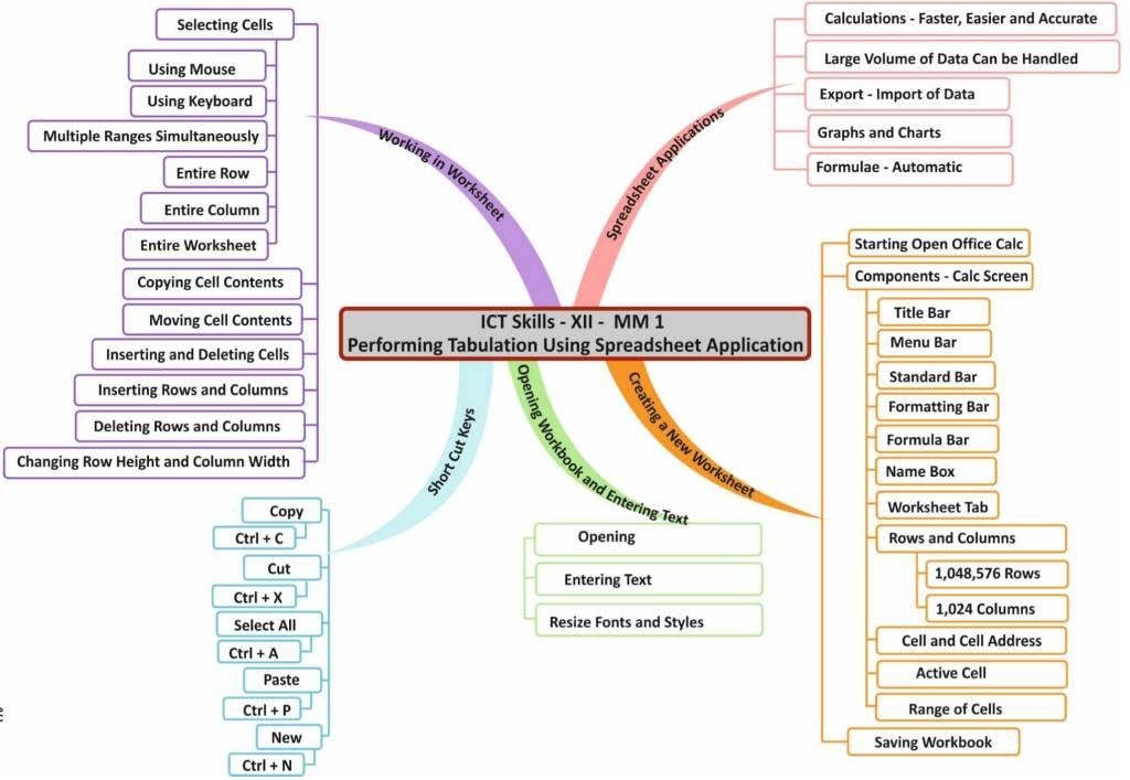
A spreadsheet programme included in the free OpenOffice Calc it a part of OpenOffice package. The majority of the capabilities found in commercial spreadsheet tools are present in this user-friendly programme. openOfficeCalc is a piece of software that assists with formula computations and data analysis.

SPREADSHEET APPLICATIONS

Spreadsheet programs have become very popular because of the following features:
• Built-in functions make calculations easier, faster, and more accurate.
• Large volumes of data can be easily handled and manipulated.
• Data can be exported to or imported from other software.
• Data can be easily represented in pictorial form like graphs or charts.
• Formulae are automatically recalculated whenever underlying data values are changed.

CREATING A NEW WORKSHEET

To start OpenOffice Calc:

Click Start ➢All Programs ➢OpenOffice 4.1.5 ➢OpenOffice Calc.
A spreadsheet workbook named Untitled1 opens up in an OpenOffice Calc application window

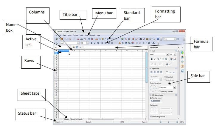
Components of a Calc Screen

Title bar
Menu bar
Standard bar
Formatting bar
Name Box
Worksheet tabs

Creating a New Workbook

The steps to create a new Calc workbook are:
Select File ➢New➢Spreadsheet.
Or
Click the New Document drop-down menu arrow on the Standard bar and selectSpreadsheet.
Or
Press CTRL + N.

Saving a workbook

Select Save option from the File menu.
Or
Click the Save icon on the Standard bar Or Press Ctrl + S
If you are saving a workbook for the first time, a Save As dialog box will appear.
2. Type the file name and choose a location to save the file. Notice that the file extension is .ods.

RESIZE FONTS AND STYLES

Selecting Cells

You can select range of cells in any one of the following ways:
• Using the mouse
• Using the keyboard

Using the mouse

To select a range of cells using the mouse, the steps are:
1. Click the cell you wish to start your selection from.
2.Click and hold the left mouse button down, drag the mouse

Using the Keyboard

To select a range of cells using the keyboard, the steps are:
1. Place the cell pointer at one of the corner cells of the range to be selected.
2. Press the SHIFT key and move to the diagonally opposite corner cell using the arrow keys.
3. Release the SHIFT key when the required range has been selected.

Copying Cell Contents

1. Select the cell(s) that contain(s) the data you want to copy.
2. Select Copy option from the Edit menu.
Or
Click the Copy button on the Standard bar.
Or
Press CTRL + C to copy the data.
3. Click on the cell(s) where you want to paste the data.
4. Select Paste option from the Edit menu.
Or
Click the Paste button on the Standard bar.
Or
Press CTRL + V.

Moving Cell Contents

To move cell contents from one cell to another in Calc, the steps are:
1. Select the cell that contains the data you want to cut.
2. Select Cut option from the Edit menu.
Or
Click the Cut button on the Standard bar.
Or
Press CTRL + X to cut the data

3. Click on the cell where you want to paste the data.
4. Select Paste option from the Edit menu.
Or
Click the Paste button on the Standard bar.
Or
Press CTRL + V.

Inserting and Deleting Cells

To insert cells, the steps are:
1. Select the range of cells where you want to insert a block of cells.
2. Select Cells option from the Insert menu.
3. The Insert Cells dialog box appears.
4. Select the appropriate option and click OK.

To delete cells, the steps are:
1. Select the range of cells where you want to delete a block of cells.
2. Select Delete Cells option from the Edit menu.
3. The Delete Cells dialog box appears.
4. Select the appropriate option and click OK.

Inserting Rows and Columns

The steps to insert rows are:
1. Select the row where you want to insert a new row.
2. Select Rows option from the Insert menu.
Or
Right-click the row header and select Insert Rows in the shortcut menu.
A new row is inserted above the selected/highlighted row.

To insert columns, the steps are:
1. Select the column where you want to insert a new column.
2. Select Columns option from the Insert menu.
Or
Right-click the column header and select Insert Columns in the shortcutmenu.

Deleting Rows and Columns

To delete rows, the steps are:

1. Select the row to be deleted.
2. Right-click on the selected row header.
3. Select Delete Rows option in the shortcut menu.
To delete multiple rows, select them using the CTRL key, or by dragging the mouse while holding the left mouse button.

To delete columns, the steps are:
1. Select the column to be deleted.
2. Right-click on the selected column header.
3. Select Delete Columns in the shortcut menu.
To delete multiple columns, select them using the CTRL key, or by dragging the mouse while holding
the left mouse button.

Changing Row Height and Column Width

You can change the row height in a Calc worksheet in any of the following ways:
• Drag the divider below the row (Fig 9).
• To fit the row height to the cell contents, double-click the divider.
• Select Format ➢Row ➢Height. The Row Height dialog box appears. Enter the value for row height in the Height spinbox. Click Ok button.

Changing Column Width

You can change the column width in a Calc worksheet in any of the following ways:
• Drag the divider to the right of the column header.
• To fit the column width to the cell contents, double-click the divider.
• To change the column width, select Format ➢Column ➢Width.
The Column Width dialog box appears. Enter the value for column width in the Width spinbox. Click Ok button.

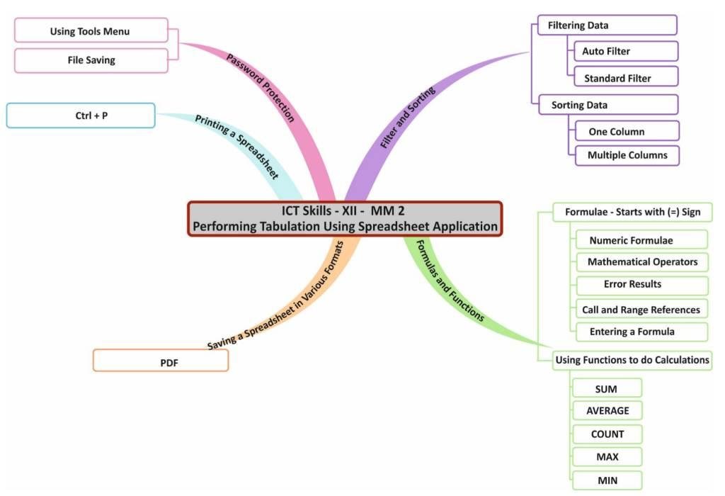
FILTER AND SORTING

Filtering Data

Based on the criteria you provide, filtering is a quick and simple approach to locate and work with selected data. Only the rows or columns that satisfy the rules or criteria you define are displayed when using the filter feature, which selectively shuts out the data you do not want to see. Filtering merely temporarily conceals the rows and columns you do not want, whereas sorting completely changes the range of cells.

Different ways in which filtering can be done in Calc are:
• AutoFilter
• Standard Filter

AutoFilter
To apply AutoFilter in a worksheet, the steps are:
1. Select cell, say, A1.
2. Select Data ➢ Filter ➢ AutoFilter.
3. A drop-down menu arrows appear in each column heading (Fig 12).
4. Click the drop-down menu arrow for Total Sales and select an item (Fig 13).
5. Only those rows whose contents meet the filter criteria are displayed.

To display all the records again, select the All option in the filter drop-down menu.
Select Top 10 to display the highest 10 values.

Standard Filter
To apply standard filter in your worksheet, the steps are:
1. Select Data➢ Filter ➢ Standard Filter..
2. The Standard Filter dialog box appears.
a. You can use the dialog box to connect multiple conditions with either a logical AND or a logical OR operator.
3. Select the options in the Standard Filter dialog box. The records with Total Sales greater than 4000 will be displayed.

Sorting Data

You can organise the data in a spreadsheet in either an ascending or descending order after entering the necessary data and using the necessary formulas. This is known as data sorting. One of the key functions of any spreadsheet software is the ability to sort on both numerical and textual values. Sorting can be done in Calc in the manner described below.

Sorting on One Column
1. Enter data in a worksheet .
2. Select any cell, say C1.
3. Click the Sort option from the Data menu, The Sort dialog box appears. Notice that column Marks appears
under Sort by section.
4. Select the Descending option under Sort by and click OK.
5. The data in column Marks is sorted in descending order.

There is a two ways to short the data in calc

Ascending
Descending

Sorting on Multiple Columns
You can sort the data on multiple columns.
1. Consider the following worksheet.
2. Select cell, say C1.
3. Select Sort option from Data menu.
4. The Sort dialog box appears.
5. The Sort Criteria tab on the Sort dialog box has options to sort the data on multiple columns.
6. Select the options.
7. The data is sorted in descending order of column

FORMULAS AND FUNCTIONS

Formulas

To compute results using arithmetic operations, formulae are utilized. In Calc, a formula always begins with the equal to (=) symbol. The formula will be interpreted as text and no computation will be made if the = sign is omitted. Additionally, nothing should be written before the = symbol. It will once more be handled as text, and no calculations will be made.

The data in a formula consists of one or a combination of the following:
Value Numeric (e.g., 45) or string (e.g., “Smiling”)
Cell Address B4, A2:C6
Function SUM, AVERAGE, MIN, MAX, etc.
Operator +, -, *, /, >, =, etc.
Parenthesis To control the left to right order of precedence in a formula (e.g., = (B2*B3)*2)

Numeric Formulae

In numeric formulae, you have to make use of operators. The results are calculated based on the order of precedence of the operators.

Mathematical Operators Used in Formulae

The mathematical operators used in Calc and their order of evaluation in formulae is given below:

Order of evaluation

Any operation contained within brackets will be carried out first
Then any exponent.
Then follow division and multiplication operations. Multiplication and division are given equal importance. They are carried out in the order they occur in the formula, from left to right. Whichever appears first in the formula is carried out first.
After that, addition and subtraction operations are given equal importance. They are also carried out in the order they occur in the formula, from left to right.

Error Results

Sometimes a formula displays an error result rather than a proper value. This happens when the formula or data has a problem and Calc cannot evaluate it.
Some common errors are shown below:

Error Reason
##### The column is not wide enough to display the value.
#DIV/0! The formula contains an invalid operation, i.e., division by zero.
#VALUE! The formula has invalid argument, e.g., text in a cell where numeric value is required.

Text Formulae

A text string or a text value is a sequence of characters. You can join two strings together. This is called concatenation. We use the ampersand (&) character to concatenate strings. For example, if you type = “Keep” &“ “& “Smiling” in a cell and press ENTER, you will see the result as Keep Smiling.

You cannot do operations such as subtraction, multiplication, and division on strings.

Cell and Range References

A cell or a group of cells are identified by a cell reference. The intersection of a row and a column gives each cell in the worksheet a unique address. Cell referencing is the practise of using a cell address in a formula.

Entering A Formula

All formulae in OpenOfficeCalc begin with an equal to (=) sign. A formula can contain number, text, arithmetic operators (+, -, *, /), or functions. The order of precedence is already discussed.
To enter a formula:
1. Select the cell and enter the formula directly in the cell or in the Formula Bar.
2. Press the Enter key.
3. The cell will show the result of the formula and the formula itself. You can see the formula in the Formula bar when the cell is selected.

Using Functions to do calculations

Functions are predefined formulae that perform calculations using specific values called arguments.

The format of writing any function in Calc is:
=function_name(Argument1;Argument2; Argument3;…..)
Arguments These are the values passed to a function so that the function carries out the intended
calculation or manipulation to give results. Arguments can be constants, formulae, or function.

SUM Function

You have already learnt how to find total using the formula. You can also obtain the sum of the values
in a range of cells by:
• Clicking the Sum button on the Formula bar (Fig 26)
• Using the SUM() function

AVERAGE Function

Average function is used to find the average of numbers in a range of cell. For example:
Formula

=AVERAGE(3;6;9)

COUNT Function

The COUNT function is used to count the number of numeric values in a range of cells. For example:
Formula

=COUNT(5;8;14;19)

MAX Function

The MAX function is used to find the maximum of numbers in a given range of cells. For example,
Formula
=MAX(74;102;134)

MIN Function

The MIN function is used to find the minimum of values in the given range of cells. For example;
Formula
=MIN(74;102;134)

PASSWORD PROTECTION

Your spreadsheet can be password-protected in OpenOffice Calc. You can either put a password on a Calc document or a sheet to safeguard your data. The Tools menu and document saving options both allow for this.

Using Tools menu

The steps to protect worksheet or Calc document using option of Tools menu are:
1. Select Tools menu ➢ Protect document Choose whether to protect Sheet or Document.
2. If you select Sheet, the Protect Sheet dialog box appears.

3. Type the password in Password text box. Again type the password in Confirm text box. Note that the password is case sensitive.
4. Click OK button

Protecting Calc doument while Saving

You can also protect your spreadsheet with a password while saving the document. The steps are:
1. Select Save As option from File menu.
2. The Save As dialog box appears. Select the drive and the folder where you want to save the file.

3. Select Save with password check box

4. Click Save button.
5. The Set Password dialog box appears.
6. Enter the password to open. Again type the password in Confirm password text box.
7. Next, click on More options. The dialog box expands
8. Here, you can give file sharing password. You can select the check box of Open file read-only option, if you want the recipient to only read the file and make no changes. You can also enter password to allow editing.
9. Click OK button.

SAVING A SPREADSHEET IN VARIOUS FORMATS

Saving in Microsoft Excel Format

If you want to save the file in the Microsoft Excel file format, then do the following while saving:
1. Select Save As option from the File emnu.
2. The Save As dialog box appears. (Fig 39)
3. Change the Save as type to Microsoft Excel 97/2000/XP(.xls).
4. Delect the drive and the folder where you want to save the file.
5. Type the filename and clcik Save button.

Saving in PDF format

The most secure method is to first save the document in the Portable Document Format (PDF) before sharing it. The easiest way to accomplish this is:

Click on the Export Directly as PDF icon on the Standard bar. This will export the entire document using the default PDF settings.
The Export dialog box appears.
Select the drive and the folder where you want to save the file.
Type the file name and click OK button.

Employability Skills Class 12 Notes

Unit 1 : Communication Skills – IV
Unit 2 : Self-Management Skills – IV
Unit 3 : Information and Communication Technology Skills – IV
Unit 4 : Entrepreneurial Skills – IV
Unit 5 : Green Skills – IV

Basic ICT Skills Class 12 Notes